Neural Networks Basics
Neural Networks Structure
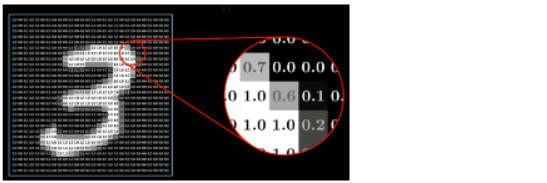
Classic example: Recognize handwritten digits represented on 28 x 28 pixel grid (Sanderson, 2017)


Figure 1. A pixel has gray value between 0.0 and 1.0 (black is 0, white is 1). Source: Sanderson, 2017.
- Pixel value determines the activation of the neuron
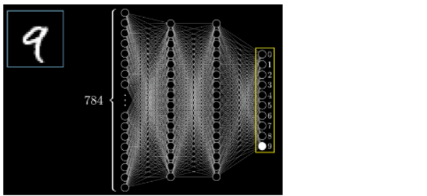
- Example of NN with 2 hidden layers of 16 neurons each
- Input layer:
- 784 (28 x 28) neurons, with activation values: a_1, a_2, a_3, …, a_784
- Two hidden layers, each of 16 neurons
- Output layer: 10 neurons
- Input layer:

 Figure 2. Neural network with 784-neuron input layer, 2 16-neuron hidden layers, and a 10-neuron output layer. Recognizing a handwritten image of the digit 9 shows 1.0 activation for the last neuron in the output layer.
How are the activations of the NEXT layer of neurons calculated?
- Sum of a_i * w_i is calculated from the input layer activations to produce the activation of each neuron on the next layer
- The weights are positive or negative numbers
- Think of the weights as strings of the connection between layers
- Subtract a bias value to the sum, representing a threshold of when the activation (the calculated sum) counts (is meaningful)
- Think of the bias as the tendency of a neuron to be connected or not
- Squish the sum to be a value between 0.0 and 1.0
- Sigmoid() function – old technology
- Rectified Linear Unit (ReLU) function - new technology
- ReLU(x) is 0 if x is negative, or ReLU(x) = x, if x is positive
- Alternative definition: ReLU(a) = max(0, a)
- Example reLU(a1w1 + a2w2 + … _ a784*w784 -B), produced an activation value between 0.0 and 1.0 for a neuron in the 1st hidden layer
- Repeat the calculation of the activations of the 16 neurons on the 2nd layer
- Repeat once more to calculate the activation of the single neuron in the output layer
- Sum of a_i * w_i is calculated from the input layer activations to produce the activation of each neuron on the next layer
What’s the total number of weights and biases in this NN (784 inputs, 2 hidden layers of 16):
- Number of weights: 78416 + 1616 + 16*10
- Number of biases: 16 + 16
- Total: 13,002
How off is the guess?
- (guess – correct)**2 is the cost of the training example
- After lots of training, we calculate the average cost
- The lower the cost, the higher the accuracy
- Accuracy: # correct guesses / # trials
- To learn: minimize the cost function
Gradient Descent Method
The problem: find all the weights to get the minimum cost
The algorithm: stochastic gradient descent
Idea: Repeatedly “nudge” the input (all the weights and biases) such that the output converges to a minimum
- The “nudging” is a multiple of a negative gradient
Visualization tool: See MLAAddict, 2023.
Least Squares Method
Idea: Given two sets of observations, find possible correlation between them
In mathematical terms, see Chalberg (2009), pages 1-2.
- Set A = {a_1, a_2, …, a_n} and set B = {b_1, b_2, …, b_n} represent n distinct quantifiable observations
- We assume a relation between each data points pair,
- a_1 and b_1, a_2 and b_2, …, of the form: a_1 * x = b_1, a_2 *x = b_2, …, expressed by the equation
- a_i * x = b_i, or its equivalent: a_i *x - b_i = 0, for every pair of corresponding observations in A and B sets
- However, real observations may have some margin of error. The equation that takes into account potential observational errors:
- a_i * x - b_i = v_i, where v_i is a real numeric value, positive or negative
- The sum of the squares of v_i estimates the overall correlation error
- Why not the sum of v_i?
- The sum of squares more accurately estimates the error because it avoids the situation of large negative and large positive errors between certain data point pairs to cancel out.
Least squares method is to minimize the sum of squares of the offsets (or residuals) between
- what’s being observed and
- the correlation that’s being estimated.
The method was invented by the Parisian mathematician Andrien-Marie Legendre in 1805 before regression analysis was formalized. The famous German mathematician Carl Friedrich Gauss also claimed that he discovered this method. Legendre did his discovery trying to predict locations of future comets based on location and trajectory data of past comets.
References
Tim Chalberg. 2009. Regression Analysis: A Powerful Tool and Riveting Drama. History of Mathematics Special Interest Group Mathematical Association of America (HOM SIGMAA) Student Paper Contest.
MLAddict. 2023. https://www.mladdict.com/linear-regression-simulator
Grant Sanderson. 2017. Neural networks from the ground up. 3Blue1Brown. https://www.3blue1brown.com/lessons/neural-networks. YouTube video https://www.youtube.com/watch?v=aircAruvnKk
More on 3Blue1Broan at https://en.wikipedia.org/wiki/3Blue1Brown#Origin.